

What This Node Does
The Forecast node generates a forward-looking projection from a historical time series using ETS (exponential smoothing, Holt-Winters). Point a date field at the Rows bucket, the metric you want to project at the Values bucket, and Go Fig fits a model and emits the forecast horizon as additional rows on the same time grain. Optionally split the series into multiple parallel forecasts by adding columns to the Columns bucket (e.g., one forecast per region, product, or customer segment).When to Use This Node
Use the Forecast node when you need to:- Project revenue or expenses for the next N months given a clean historical series
- Forecast unit sales by SKU or region in parallel using a single node
- Build budget-vs-forecast comparisons in a flow that already aggregates actuals
- Stress-test a baseline by toggling trend and seasonality components
Step-by-Step Usage Guide
1
Configure the buckets
- Rows: the date field to forecast over (typically
month,week, orday). - Values: the numeric field to forecast (e.g.,
revenue,units_sold). Pick an aggregation function (Sum is most common). - Columns (optional): dimension(s) to fit one independent model per group, e.g.,
regionto get separate forecasts per region in parallel.
2
Set the forecast horizon
Enter the number of periods to forecast in the Forecast Horizon field. Units match the date grain in the Rows bucket: 6 with monthly data = 6 months ahead. Range: 1 to 365.
3
Choose a growth pattern
The Growth Pattern setting controls how the trend component is modeled:
- Linear (default): additive trend. Use for series with steady absolute growth (e.g., +$50K/month).
- Exponential: multiplicative trend. Use for series growing as a percentage (e.g., +5%/month).
- None: no trend component. Use for stable series with no directional drift.
4
Choose a seasonal pattern
The Seasonal Pattern setting controls how recurring cycles are modeled:
- Consistent (default): additive seasonality. Use when seasonal swings are similar in absolute size each year (e.g., December always +$200K).
- Proportional: multiplicative seasonality. Use when seasonal swings scale with the level of the series (e.g., December is always 30% above average).
- None: no seasonal component. Use for short series (< 2 full cycles) or non-seasonal data.
5
Run and inspect
Run the node. Output extends the input table with 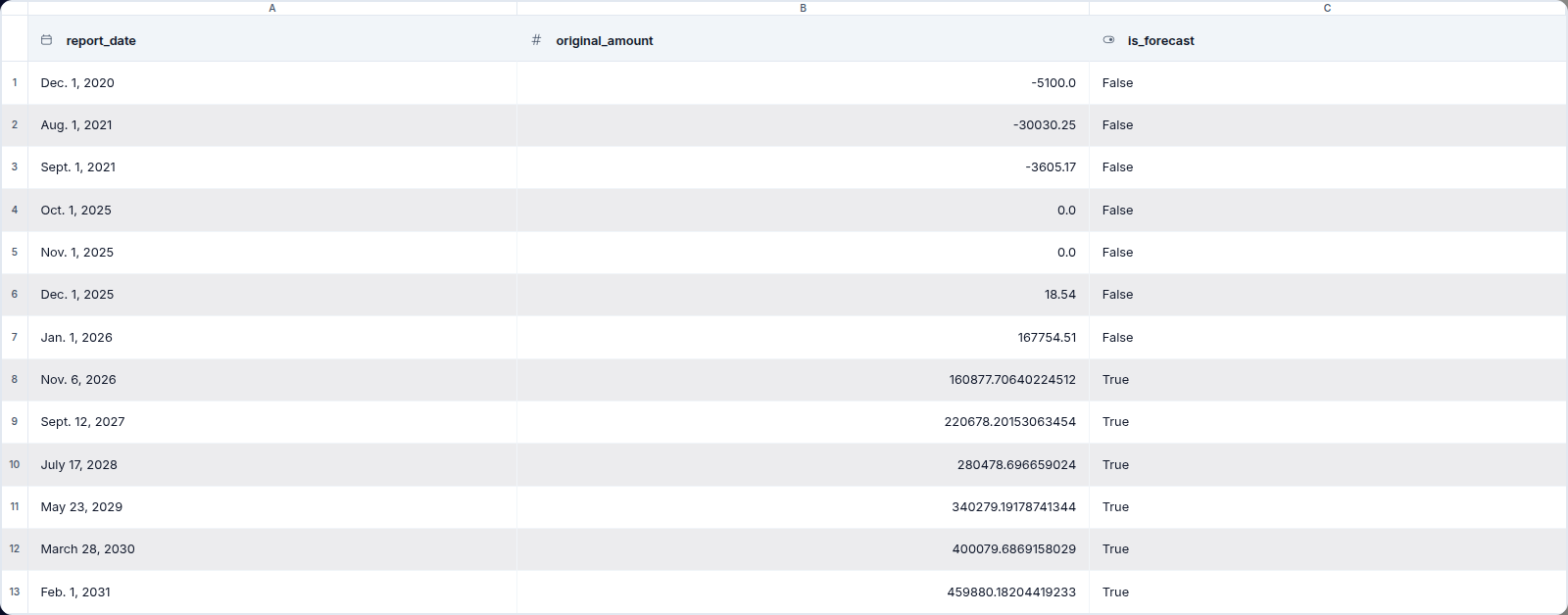
periods additional rows. Forecast values appear in the same Values field. A generated is_forecast boolean field distinguishes actuals from projections.